5 Linear Models

5.1 Topic 1 (BV)

Getting Started

5.2 Sums of Squares Types

Getting Started

To demonstrate the various types of sums of squares, we’ll create a data frame called df_disease taken from the SAS documentation (reference). The summary of the data is shown.

## # A tibble: 3 x 3
##   drug  disease     y
##   <fct> <fct>   <dbl>
## 1 1     1          42
## 2 1     1          44
## 3 1     1          36

##  drug   disease       y        
##  1:18   1:24    Min.   :-6.00  
##  2:18   2:24    1st Qu.: 9.00  
##  3:18   3:24    Median :21.00  
##  4:18           Mean   :18.88  
##                 3rd Qu.:28.00  
##                 Max.   :44.00  
##                 NA's   :14

The Model

For this example, we’re testing for a significant difference in stem_length using ANOVA. In R, we’re using lm() to run the ANOVA, and then using broom::glance() and broom::tidy() to view the results in a table format.

lm_model <- lm(y ~ drug + disease + drug*disease, df_disease)

The glance function gives us a summary of the model diagnostic values.

lm_model %>% glance()

## # A tibble: 1 x 12
##   r.squared adj.r.squared sigma statistic p.value    df logLik   AIC   BIC
##       <dbl>         <dbl> <dbl>     <dbl>   <dbl> <dbl>  <dbl> <dbl> <dbl>
## 1     0.456         0.326  10.5      3.51 0.00130    11  -212.  450.  477.
## # ... with 3 more variables: deviance <dbl>, df.residual <int>, nobs <int>

The tidy function gives a summary of the model results.

lm_model %>% tidy()

## # A tibble: 12 x 5
##    term           estimate std.error statistic      p.value
##    <chr>             <dbl>     <dbl>     <dbl>        <dbl>
##  1 (Intercept)      29.3        4.29    6.84   0.0000000160
##  2 drug2            -1.33       6.36   -0.210  0.835       
##  3 drug3           -13.0        7.43   -1.75   0.0869      
##  4 drug4           -15.7        6.36   -2.47   0.0172      
##  5 disease2         -1.08       6.78   -0.160  0.874       
##  6 disease3         -8.93       6.36   -1.40   0.167       
##  7 drug2:disease2    6.58       9.78    0.673  0.504       
##  8 drug3:disease2  -10.9       10.2    -1.06   0.295       
##  9 drug4:disease2    0.317      9.30    0.0340 0.973       
## 10 drug2:disease3   -0.900      9.00   -0.100  0.921       
## 11 drug3:disease3    1.10      10.2     0.107  0.915       
## 12 drug4:disease3    9.53       9.20    1.04   0.306

The Results

You’ll see that R print the individual results for each level of the drug and disease interaction. We can get the combined F table in R using the anova() function on the model object.

lm_model %>% 
  anova() %>% 
  tidy() %>% 
  kable()

term	df	sumsq	meansq	statistic	p.value
drug	3	3133.2385	1044.4128	9.455761	0.0000558
disease	2	418.8337	209.4169	1.895990	0.1617201
drug:disease	6	707.2663	117.8777	1.067225	0.3958458
Residuals	46	5080.8167	110.4525	NA	NA

And with some extra work, we can get a Total row to match the F table output by SAS.

lm_model %>%
  anova() %>%
  tidy() %>%
  add_row(term = "Total", df = sum(.$df), sumsq = sum(.$sumsq)) %>% 
  kable()

term	df	sumsq	meansq	statistic	p.value
drug	3	3133.2385	1044.4128	9.455761	0.0000558
disease	2	418.8337	209.4169	1.895990	0.1617201
drug:disease	6	707.2663	117.8777	1.067225	0.3958458
Residuals	46	5080.8167	110.4525	NA	NA
Total	57	9340.1552	NA	NA	NA

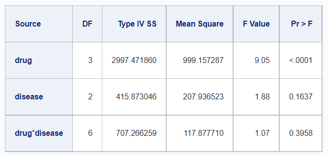
Comparing this to the output in SAS, we see the following.

proc glm;
   class drug disease;
   model y=drug disease drug*disease / ss1 ss2 ss3 ss4;
run;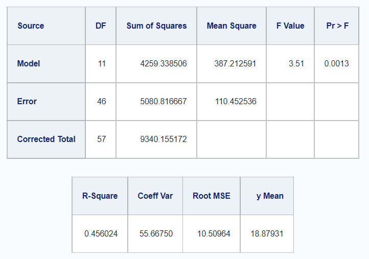

Sums of Squares Tables

In SAS, it is easy to find the tables for the variouse types of sums of squares calculations. Unfortunately, it is not easy to match this output in using functions from base R. However, the rstatix package offers a solution to produce these various sums of squares tables. Note that there does not appear to be a Type IV SS equivalent in R.

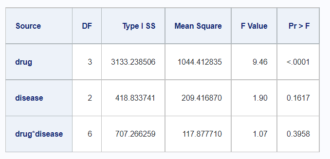
5.2.0.1 Type I

In R,

df_disease %>% 
  rstatix::anova_test(
    y ~ drug + disease + drug*disease, 
    type = 1, 
    detailed = TRUE) %>% 
  rstatix::get_anova_table() %>% 
  kable()

Effect	DFn	DFd	SSn	SSd	F	p	p<.05	ges
drug	3	46	3133.239	5080.817	9.456	5.58e-05	*	0.381
disease	2	46	418.834	5080.817	1.896	1.62e-01		0.076
drug:disease	6	46	707.266	5080.817	1.067	3.96e-01		0.122

And in SAS,

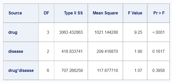
Type II

In R,

df_disease %>% 
  rstatix::anova_test(
    y ~ drug + disease + drug*disease, 
    type = 2, 
    detailed = TRUE) %>% 
  rstatix::get_anova_table() %>% 
  kable()

Effect	SSn	SSd	DFn	DFd	F	p	p<.05	ges
drug	3063.433	5080.817	3	46	9.245	6.75e-05	*	0.376
disease	418.834	5080.817	2	46	1.896	1.62e-01		0.076
drug:disease	707.266	5080.817	6	46	1.067	3.96e-01		0.122

And in SAS,

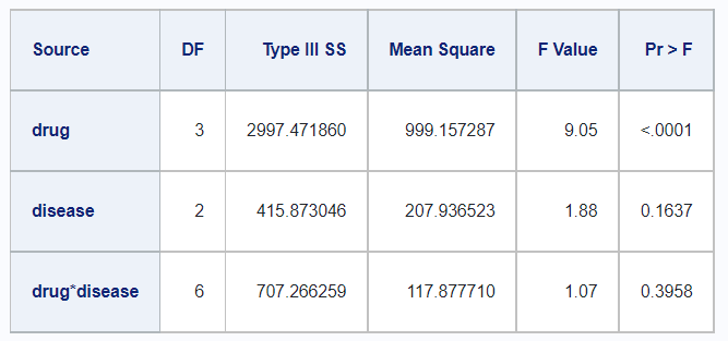
Type III

In R,

df_disease %>% 
  rstatix::anova_test(
    y ~ drug + disease + drug*disease, 
    type = 3, 
    detailed = TRUE) %>% 
  rstatix::get_anova_table() %>% 
  kable()

Effect	SSn	SSd	DFn	DFd	F	p	p<.05	ges
(Intercept)	20037.613	5080.817	1	46	181.414	0.00e+00	*	0.798
drug	2997.472	5080.817	3	46	9.046	8.09e-05	*	0.371
disease	415.873	5080.817	2	46	1.883	1.64e-01		0.076
drug:disease	707.266	5080.817	6	46	1.067	3.96e-01		0.122

And in SAS,

Type IV

In SAS,

In R there is no equivalent operation to the Type IV sums of squares calculation in SAS.

5.3 Contrasts

Getting Started

To demonstrate contrasts, we’ll create a data frame called df_trial. We see that the drug variable has three levels, A, C and E.

##  drug        pre             post       sex   
##  A:10   Min.   : 3.00   Min.   : 0.00   M:15  
##  C:10   1st Qu.: 7.00   1st Qu.: 2.00   F:15  
##  E:10   Median :10.50   Median : 7.00         
##         Mean   :10.73   Mean   : 7.90         
##         3rd Qu.:13.75   3rd Qu.:12.75         
##         Max.   :21.00   Max.   :23.00

## Rows: 30
## Columns: 4
## $ drug <fct> A, A, A, A, A, A, A, A, A, A, C, C, C, C, C, C, C, C, C, C, E, E,~
## $ pre  <dbl> 11, 8, 5, 14, 19, 6, 10, 6, 11, 3, 6, 6, 7, 8, 18, 8, 19, 8, 5, 1~
## $ post <dbl> 6, 0, 2, 8, 11, 4, 13, 1, 8, 0, 0, 2, 3, 1, 18, 4, 14, 9, 1, 9, 1~
## $ sex  <fct> M, F, M, F, M, F, M, F, M, F, M, F, M, F, M, F, M, F, M, F, M, F,~

In order to work with these levels as contrasts, we can use one of the pre-existing R functions to create the identity matrix for this factor variable. The contr.treatment definition is the default one that R uses, while the contr.SAS is the definition that SAS uses by default.

contr.treatment(levels_drug)

##   C E
## A 0 0
## C 1 0
## E 0 1

contr.SAS(levels_drug)

##   A C
## A 1 0
## C 0 1
## E 0 0

R also has the following definitions ready for use: contr.sum, contr.poly, and contr.helmert.

Using Contrasts in R

There are many ways to work with contrasts in R, but here we’re only going to focus on defining contrasts in the modeling function. In this example, we’re creating a linear model to predict post values from the pre and drug values. The only difference between the two is in the contrasts argument. In one case, we’re using the R default, and in the other we’re using the SAS default.

model_trt <- 
  lm(post ~ pre + drug, data = df_trial,
     contrasts = list(drug = contr.treatment))

model_sas <- 
  lm(post ~ pre + drug, data = df_trial,
     contrasts = list(drug = contr.SAS))

Comparing the output for these two models, we see that differ in which drug level is being used as the reference baseline.

tidy(model_trt)

## # A tibble: 4 x 5
##   term        estimate std.error statistic    p.value
##   <chr>          <dbl>     <dbl>     <dbl>      <dbl>
## 1 (Intercept)   -3.88      1.99    -1.95   0.0616    
## 2 pre            0.987     0.164    6.00   0.00000245
## 3 drug2          0.109     1.80     0.0607 0.952     
## 4 drug3          3.45      1.89     1.83   0.0793

tidy(model_sas)

## # A tibble: 4 x 5
##   term        estimate std.error statistic    p.value
##   <chr>          <dbl>     <dbl>     <dbl>      <dbl>
## 1 (Intercept)   -0.435     2.47     -0.176 0.862     
## 2 pre            0.987     0.164     6.00  0.00000245
## 3 drug1         -3.45      1.89     -1.83  0.0793    
## 4 drug2         -3.34      1.85     -1.80  0.0835

We can define a custom contrast as well. In this case, we are comparing A to E, where E is the baseline group. As is typical of contrasts, the values must sum to 0, where negative numbers represent the baseline groups.

lm(post ~ pre + drug, data = df_trial,
   constrasts = list(drug = c("A" = 1, "C" = "0", "E" = -1)))

It is possible to combine contrasts using cbind. Notice here that contrast definitions don’t require level names to be assigned, as long as the order of the levels is maintained.

contrast_1 <- c(1,  0, -1)
contrast_2 <- c(1, -2,  1)

contrast_c <- cbind(contrast_1, contrast_2)

lm(post ~ pre + drug, data = df_trial,
   contrasts = contrast_c)

Easy Contrasts in R with `emmeans`

The emmeans package makes working with contrasts much easier. In fact, this is the method that we recommend when trying to match contrast output between SAS and R.

We begin by defining some models.

model_lm <-  lm(post ~ pre + drug + sex, data = df_trial)
model_av <- aov(post ~ pre + drug + sex, data = df_trial)
model_gm <- glm(post ~ pre + drug + sex, data = df_trial)

Then we convert these models to emmeans models. In the emmeans function we can specify which variables we want to display estimated marginal means for.

model_lm %>% emmeans(specs = "drug")
model_av %>% emmeans(specs = "drug", by = "sex")
model_gm %>% emmeans(specs = ~ drug | sex)

Or, we can define some common contrasts with the contrast function.

# All Pairwise Comparisons
model_lm %>% 
  emmeans("drug") %>% 
  contrast(method = "pairwise")     

# Treatment v Control Comparison
model_gm %>% 
  emmeans("drug") %>% 
  contrast(method = "trt.vs.ctrl")

We can also control the reference group, or reverse the contrast order using the arguments in the contrast function.

model_lm %>% 
  emmeans("drug") %>% 
  contrast(method = "trt.vs.ctrl", ref = 2)     

model_lm %>% 
  emmeans("drug") %>% 
  contrast(method = "trt.vs.ctrl", rev = T)

Custom contrasts can be defined as well.

model_lm %>% 
  emmeans("drug") %>% 
  contrast(method = list(
    "A v E"  = c("A" = 1, "C" = 0, "E" = -1),
    "AE v C" = c(1, -2, 1),
    "A"      = c(1, 0, 0)
  ))

Matching Contrasts: R and SAS

It is recommended to use the emmeans package when attempting to match contrasts between R and SAS. In SAS, all contrasts must be manually defined, whereas in R, we have many ways to use pre-existing contrast definitions. The emmeans package makes simplifies this process, and provides syntax that is similar to the syntax of SAS.

This is how we would define a contrast in SAS.

# In SAS
proc glm data=work.mycsv;
   class drug;
   model post = drug pre / solution;
   estimate 'C vs A'  drug -1  1 0;
   estimate 'E vs CA' drug -1 -1 2;
run;

And this is how we would define the same contrast in R, using the emmeans package.

lm(formula = post ~ pre + drug, data = df_trial) %>% 
  emmeans("drug") %>% 
  contrast(method = list(
    "C vs A"  = c(-1,  1, 0),
    "E vs CA" = c(-1, -1, 2)
  ))

Note, however, that there are some cases where the scale of the parameter estimates between SAS and R is off, though the test statistics and p-values are identical. In these cases, we can adjust the SAS code to include a divisor. As far as we can tell, this difference only occurs when using the predefined Base R contrast methods like contr.helmert.

proc glm data=work.mycsv;
   class drug;
   model post = drug pre / solution;
   estimate 'C vs A'  drug -1  1 0 / divisor = 2;
   estimate 'E vs CA' drug -1 -1 2 / divisor = 6;
run;

4 Summary Statistics

6 Mixed Models

5 Linear Models

5.1 Topic 1 (BV)

Getting Started

5.2 Sums of Squares Types

Getting Started

The Model

The Results

Sums of Squares Tables

5.2.0.1 Type I

Type II

Type III

Type IV

5.3 Contrasts

Getting Started

Using Contrasts in R

Easy Contrasts in R with emmeans

Matching Contrasts: R and SAS

Easy Contrasts in R with `emmeans`