6 Mixed Models

6.1 Repeated Measures

6.1.1 Introduction

This document focuses on a comparison of results generated using a Mixed Model for Repeated Measures (MMRM) in SAS and R. Data for the comparison was the lab ADaM dataset adlbh.xpt from the Phuse Pilot Study. Results were generated for each lab parameter and time point in the dataset using three different covariance structures, i.e. unstructured, compound symmetry and autoregressive of first order (AR(1)).

6.1.1.1 Fitting the MMRM in SAS

In SAS the following code was used (assessments at avisitn=0 should also be removed from the response variable):

proc mixed data=adlbh;
where base ne . and avisitn not in (., 99);
class usubjid trtpn(ref="0") avisitn;
by paramcd param;
model chg=base trtpn avisitn  trtpn*avisitn / solution cl alpha=0.05 ddfm=KR;
repeated avisitn/subject=usubjid type=&covar;
lsmeans trtpn * avisitn / diff cl slice=avisitn;
lsmeans trtpn / diff cl;
run;

where the macro variable covar could be UN, CS or AR(1). The results were stored in .csv files that were post-processed in R and compared with the results from R.

6.1.2 Fitting the MMRM in R

6.1.2.1 Using the `nlme::gls` function

The code below implements an MMRM fit in R with the nlme::gls function.

gls(model = CHG ~ TRTP + AVISITN + TRTP:AVISITN + AVISITN + BASE,
    data = data,
    correlation = corSymm(form = ~1|SUBJID),
    weights = varIdent(form = ~1|AVISITN),
    control = glsControl(opt = "optim"),
    method = "REML",
    na.action = "na.omit")

here we can swap out corSymm for corCompSymm to give the compound symmetry structure or corCAR1 for autoregressive of first order (AR(1)).

6.1.2.2 Using the `lme4::lmer` function

An alternative way to fit an MMRM with unstructured covariance matrices is to use the lme4::lmer function as described by Daniel Sabanes Bove in his R in Pharma talk from 2020 see here. The relevance of this fit is apparent when we consider the availability of the Kenward-Roger’s degrees of freedom for the MMRM in R, which at the time of writing, were not yet available for the nlme::gls function via the pbkrtest package (see here).

lmer(CHG ~ TRTA * VISIT + VISIT + BASE + (0 + VISIT|SUBJID),
     data = data,
     control = lmerControl(check.nobs.vs.nRE = "ignore"),
     na.action = na.omit)

6.1.2.3 Extracting effect estimates using `emmeans`

In order to extract relevant marginal means (LSmeans) and contrasts we can use the emmeans package. Below we start by constructing a ref_grid used to make explicit just how the predictions are generated across the levels of TRTP and AVISITN. The emmeans function permits various marginal means to be extracted depending on the formula provided and the following pairs() function call derives relevant contrasts. Note that more control can be obtained by calling the contrast() function.

mod_grid <- ref_grid(model, data = data, mode = "df.error")
mod_emm <- emmeans(mod_grid, ~TRTP * AVISITN, mode = "df.error") 
pairs(mod_emm)

6.1.3 Comparison between SAS and R

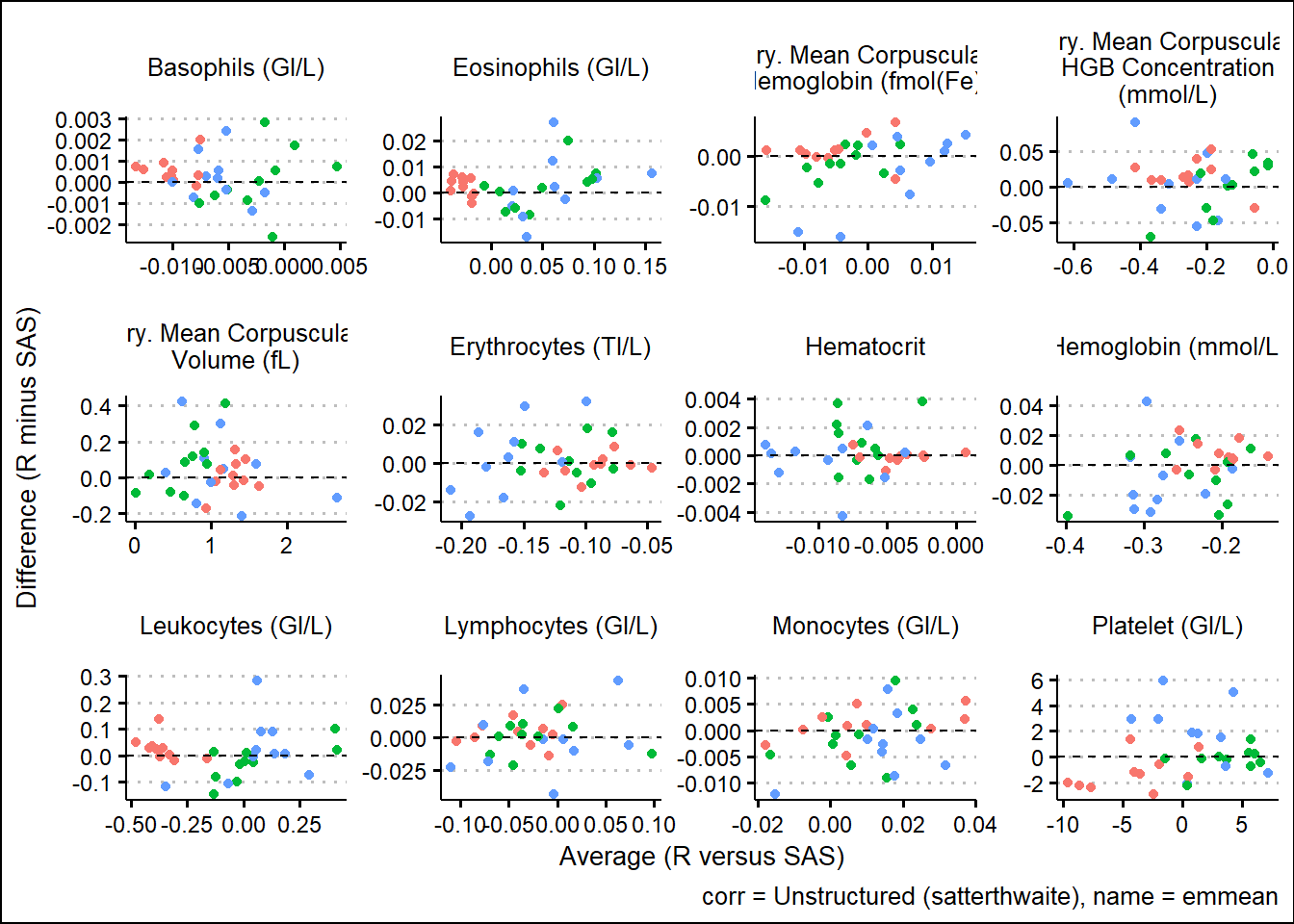
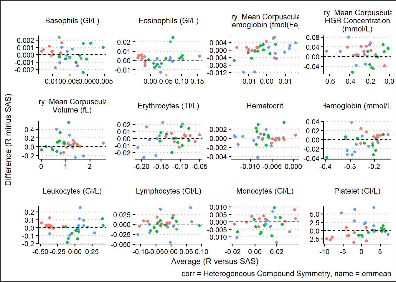
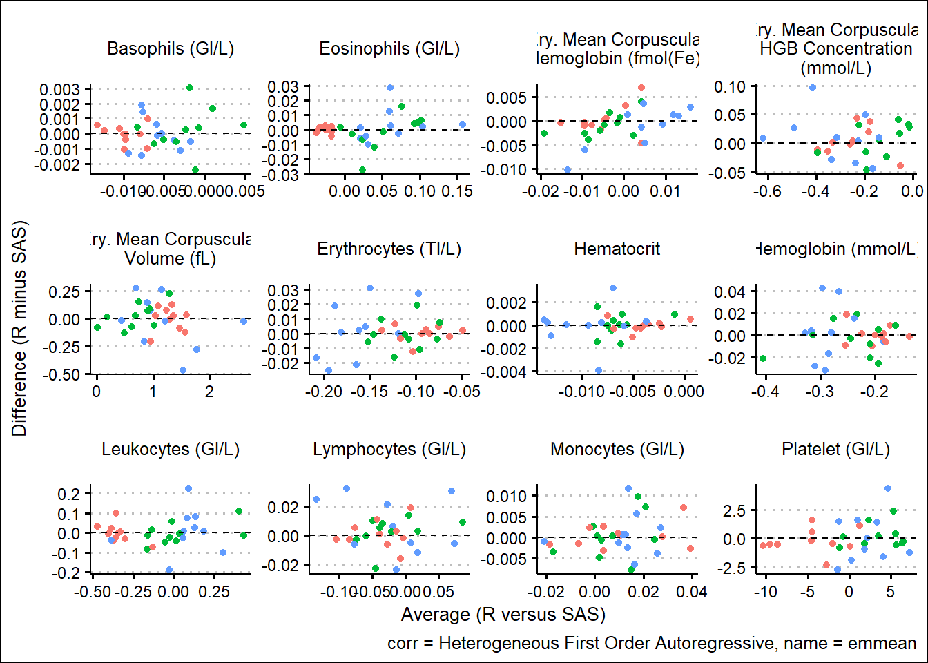
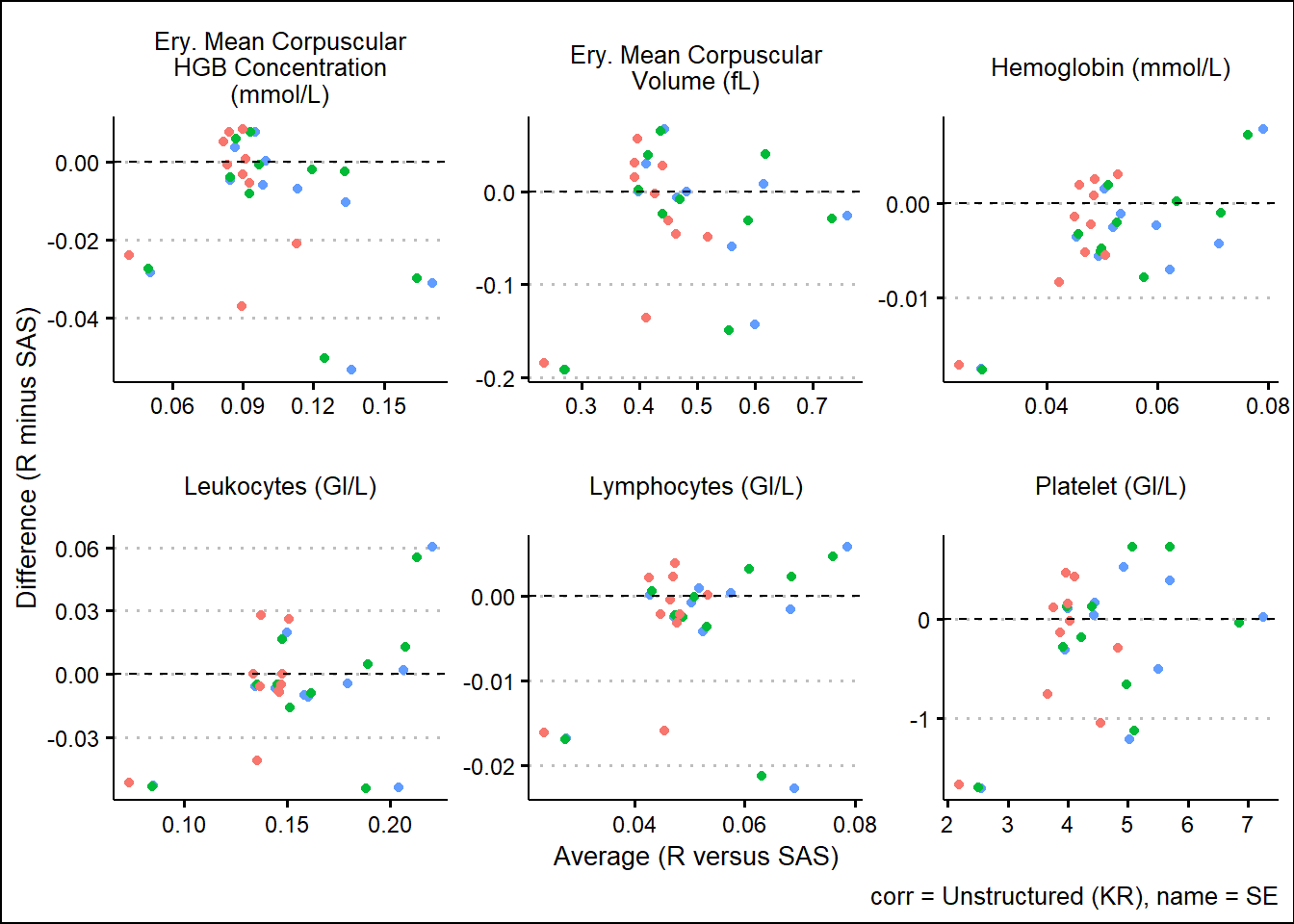
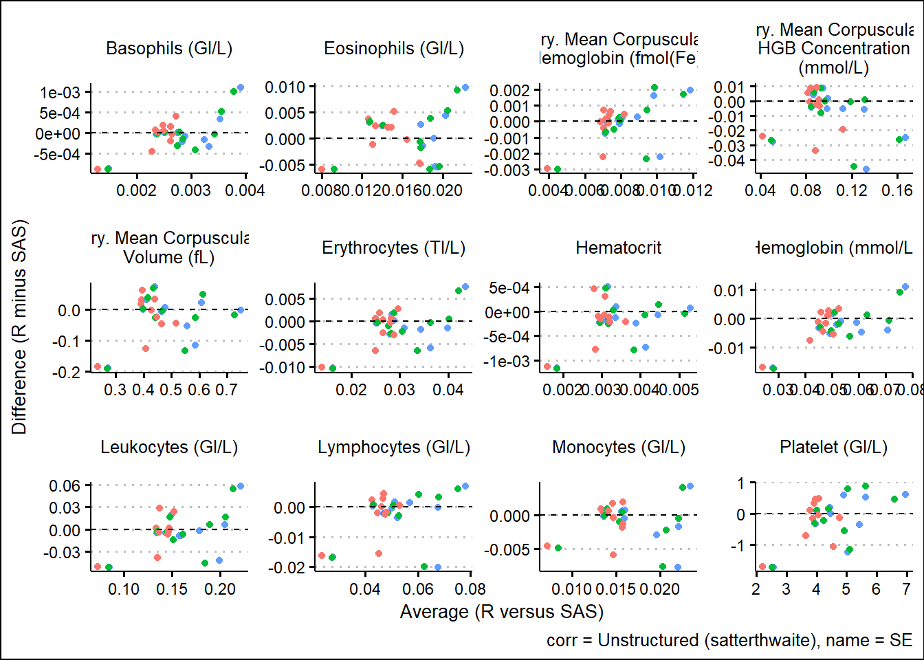
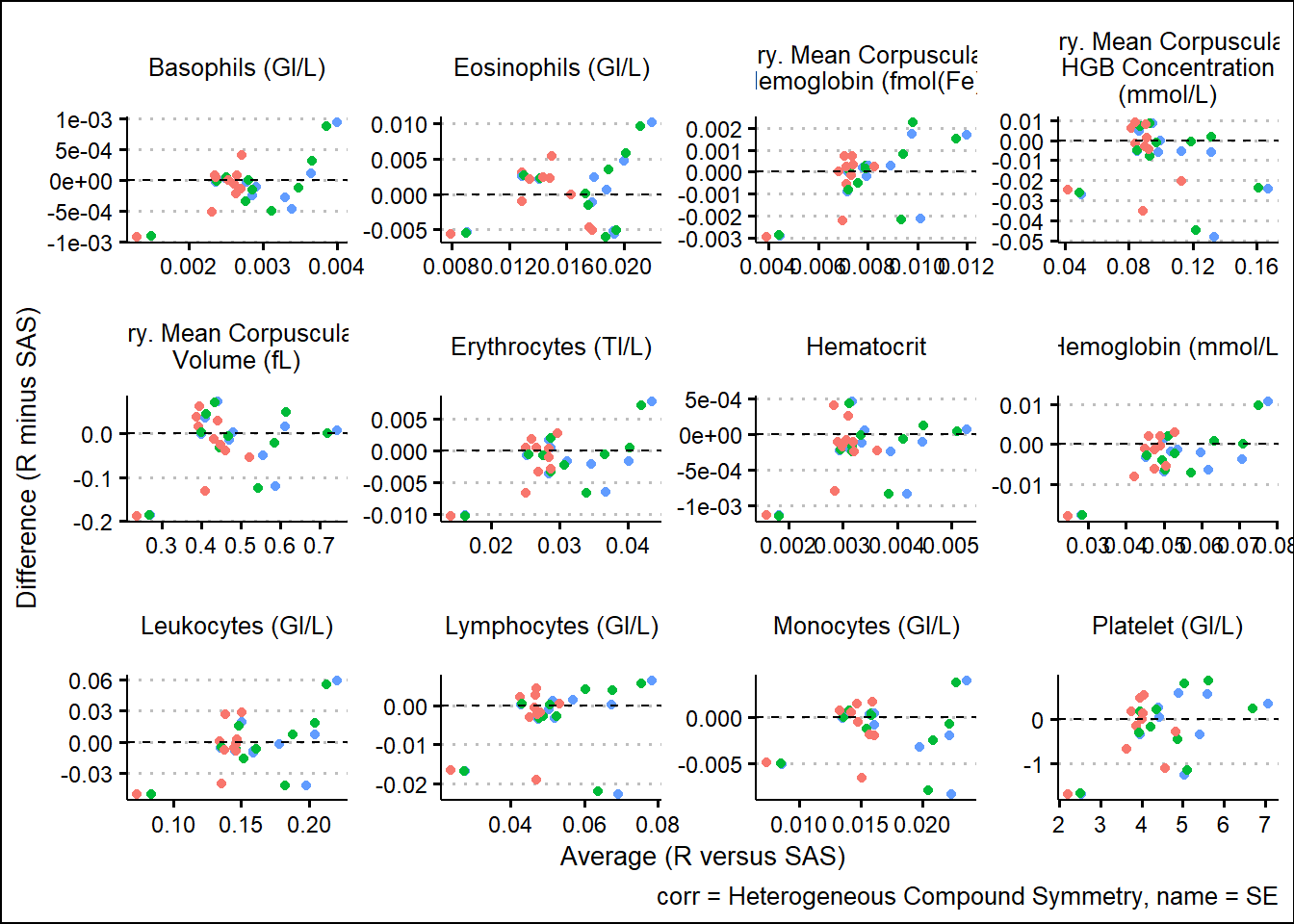
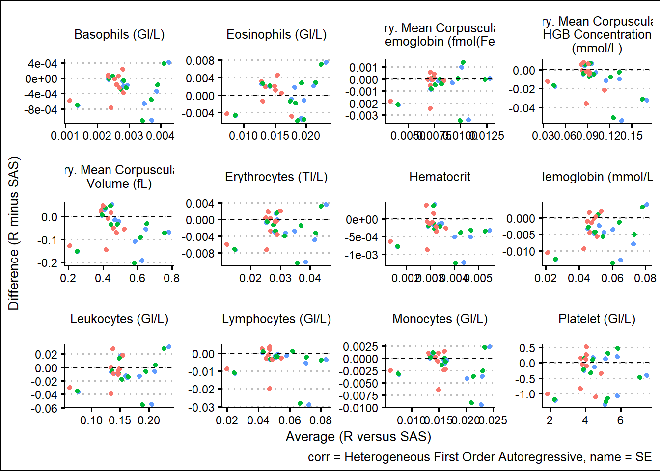
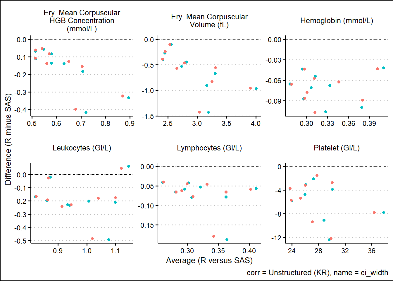
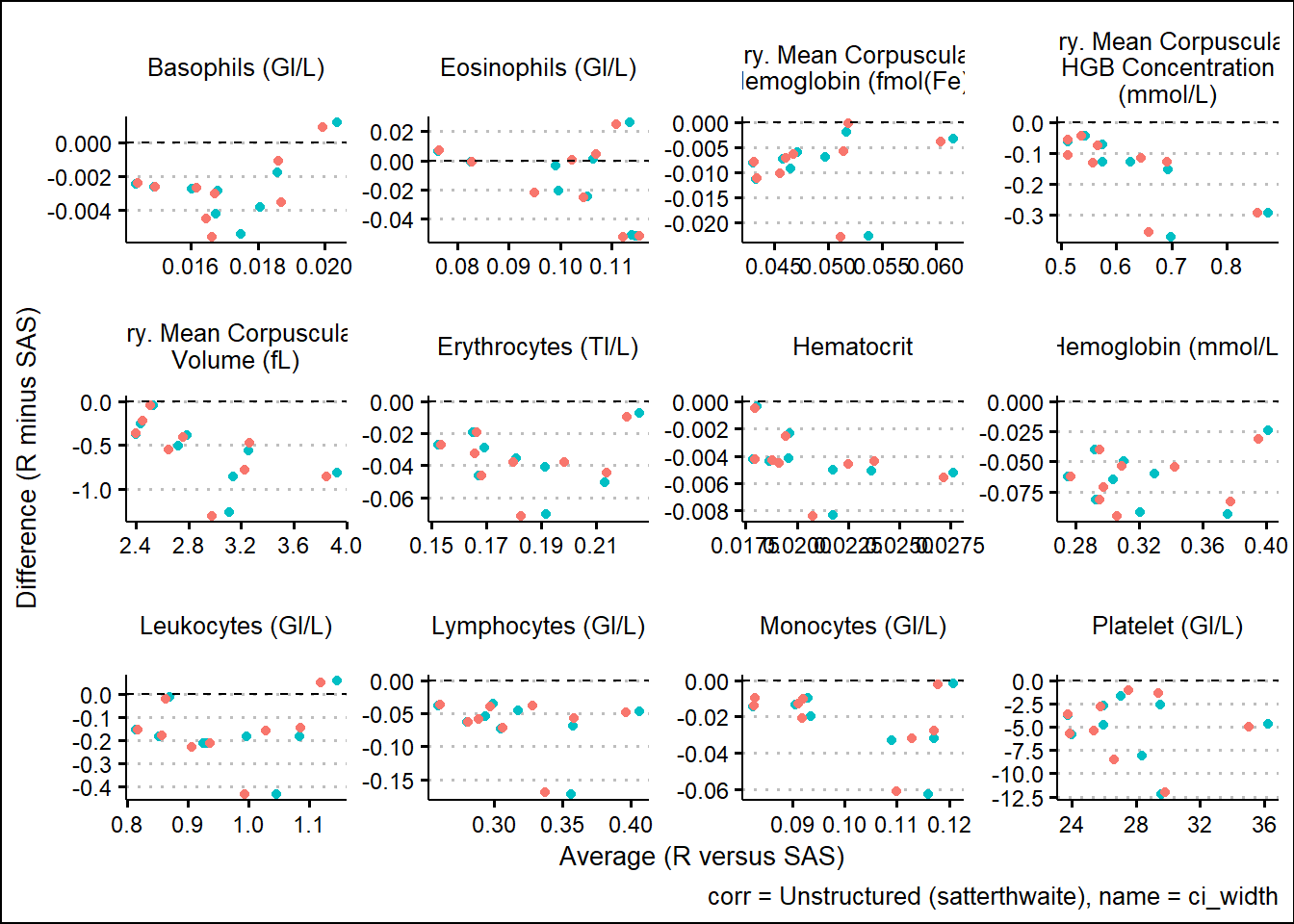
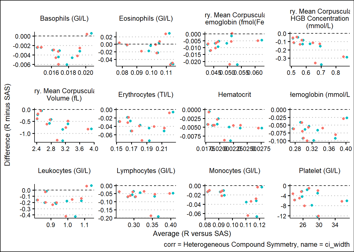
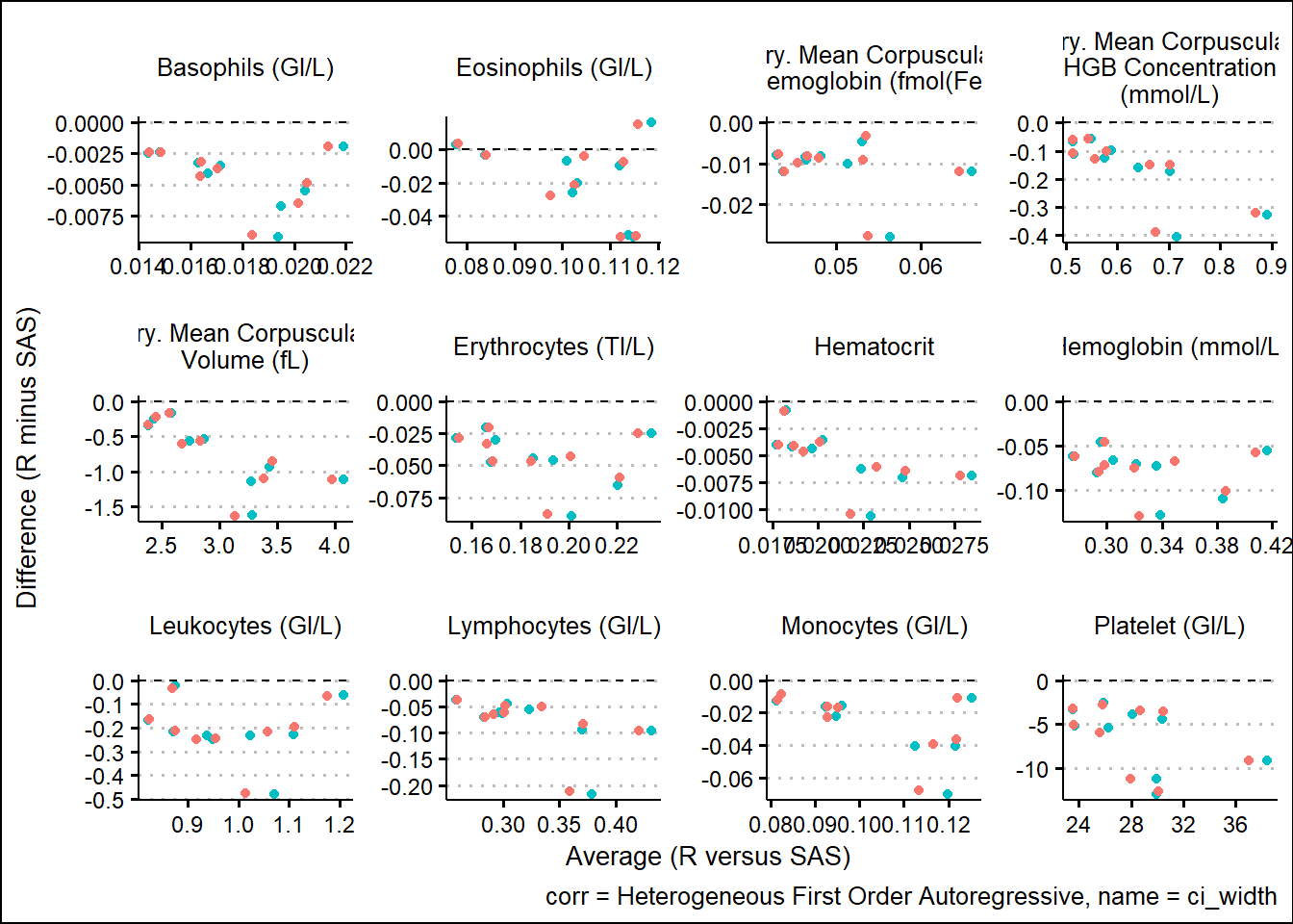
With results available for SAS and R model fits, we turn our attention to generating some visual comparisons of the results. Note that here we adopt a Bland-Altman type plot which plots the difference on the y-axis and the average on the x-axis. This offers a way to inspect any bias or relationships with the size of effect and the associated bias.

For the extracted LS-means

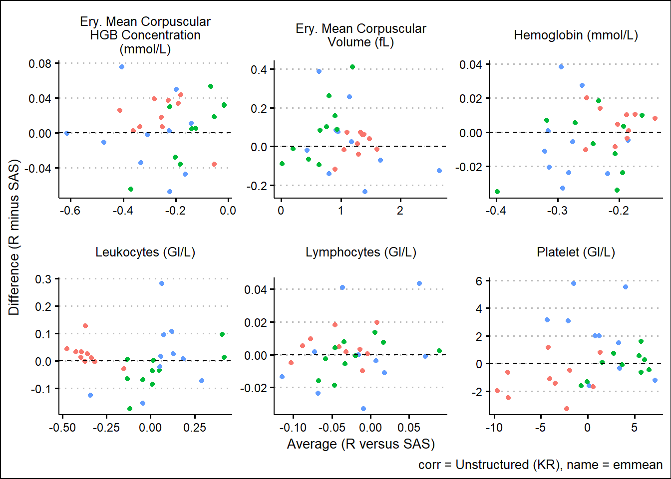
and corresponding SEs

For the derived contrasts

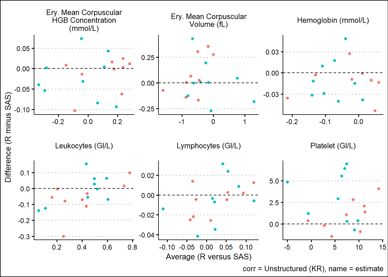
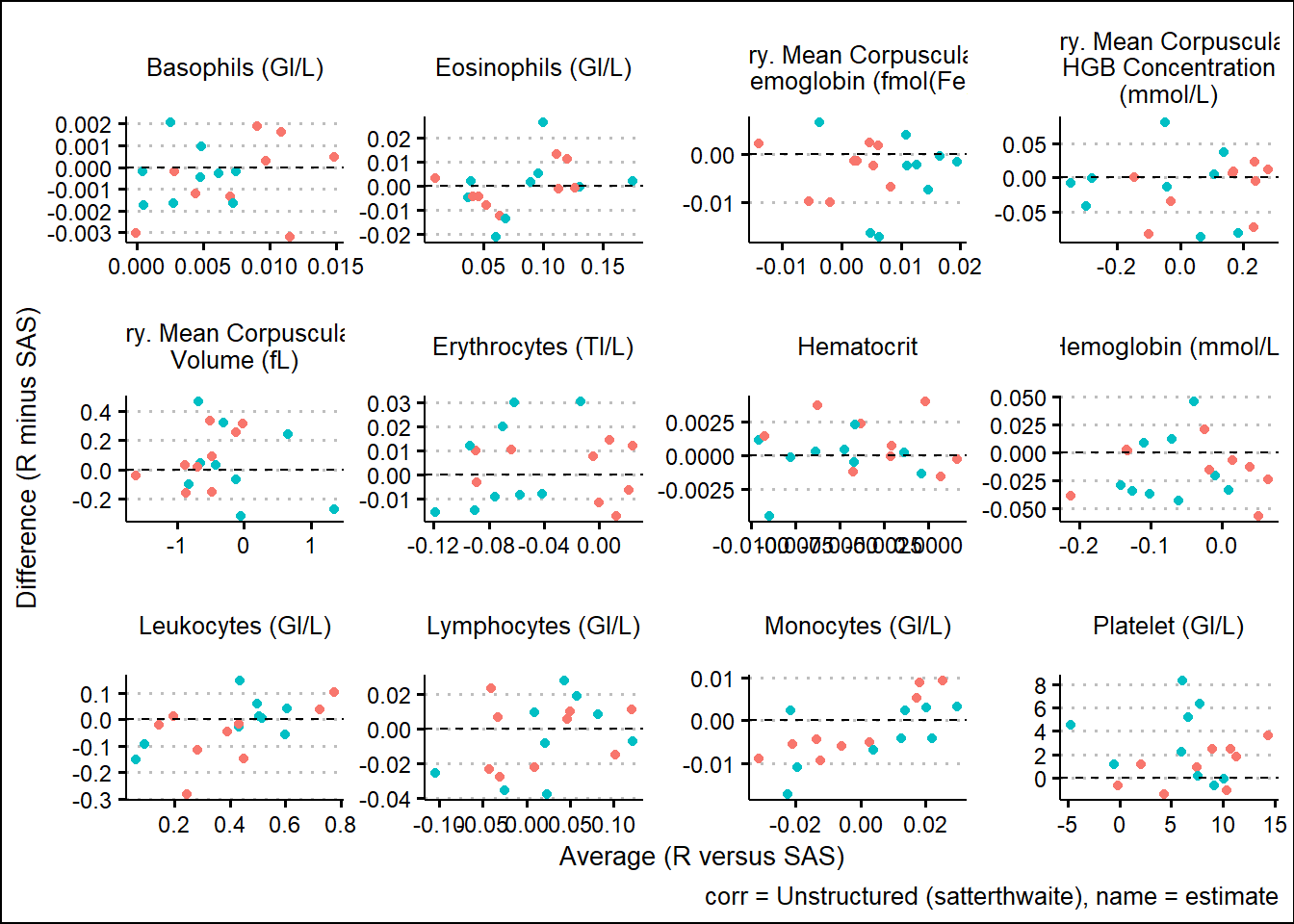
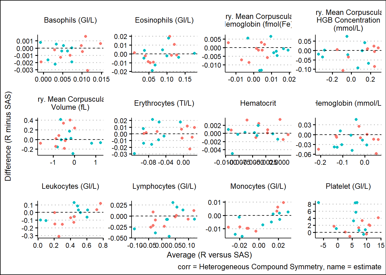
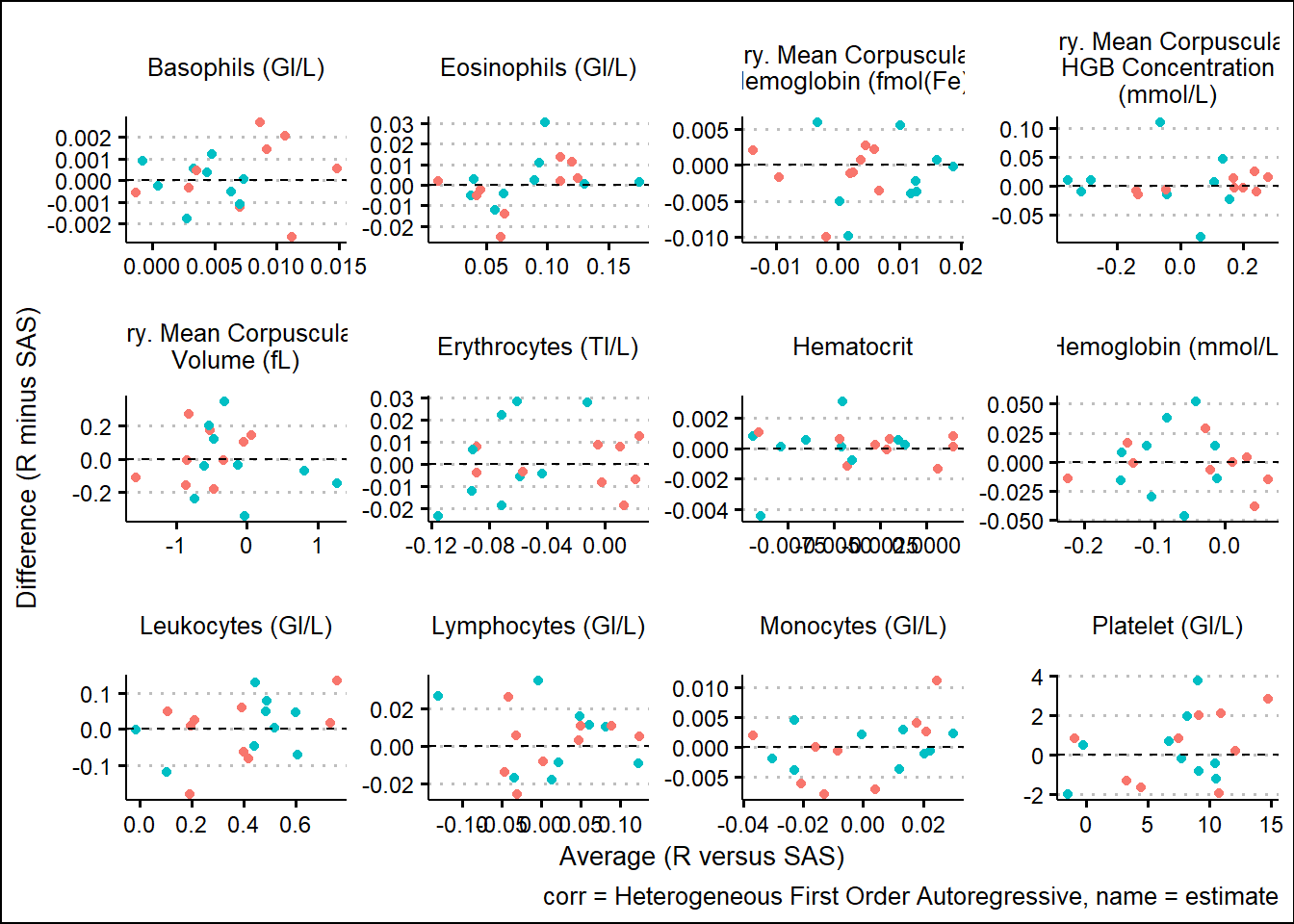
and corresponding 95%CI widths

6.1.4 Analysis of SAS and R Comparison

Using SAS PROC MIXED and R functions such as gls, lmer, mod_grid, and mod_emm, results were broadly aligned. Results not being exact can be attributed to many factors such as rounding precision, data handling, and many other internal processing nuances. However, Bland-Altman type plots showed small but randomly distributed differences across a broad range of parameters from the input data. Apart from a small subset of the parameters, there were no trends observed which would have suggested systemic differences between the languages. These analyses were based on a single set of data so more research must be done. However, based on comparing R documentation with SAS documentation, as well as the results displayed above in this paper, it is evident that the R and the SAS methods cover do produce similarly valid results for the options which were tested.

6.1.5 Future work

Run SAS code by also removing assessments at avisitn=0 from the response variable, and using trtp (or trtpn) and avisit (or avisitn)
Investigating the differences
Implement lmer equivalent to MMRM with compound symmetry
Comparisons for other models, i.e. only random, random and repeated, no repeated

5 Linear Models

7 Survival Models